MFDFA’s documentation¶

MFDFA is a python implementation of Multifractal Detrended Fluctuation Analysis, first developed by by Peng et al. ¹ and later extended to study multifractality MFDFA by Kandelhardt et al. ².

Installation¶

MFDFA is available from PyPI, so you can use

pip install MFDFA

Then on your favourite editor just use

from MFDFA import MFDFA

Warning

To use the extension to include Empirical Mode Decomposition detrending you will also need

pip install EMD-signal

An exemplary one-dimensional fractional Ornstein–Uhlenbeck process¶

For a more detailed explanation on how to integrate an Ornstein–Uhlenbeck process, see the kramersmoyal’s package You can also follow the fOU.ipynb

Generating a fractional Ornstein–Uhlenbeck process¶

This is one method of generating a (fractional) Ornstein–Uhlenbeck process with $H=0.7$, employing a simple Euler–Maruyama integration method

# Imports
from MFDFA import MFDFA
from MFDFA import fgn
# where this second library is to generate fractional Gaussian noises

# integration time and time sampling
t_final = 500
delta_t = 0.001

# Some drift theta and diffusion sigma parameters
theta = 0.3
sigma = 0.1

# The time array of the trajectory
time = np.arange(0, t_final, delta_t)

# The fractional Gaussian noise
H = 0.7
dB = (t_final ** H) * fgn(N = time.size, H = H)

# Initialise the array y
y = np.zeros([time.size])

# Integrate the process
for i in range(1, time.size):
   y[i] = y[i-1] - theta * y[i-1] * delta_t + sigma * dB[i]

And now you have a fractional process with a self-similarity exponent $H=0.7$

Using the `MFDFA`¶

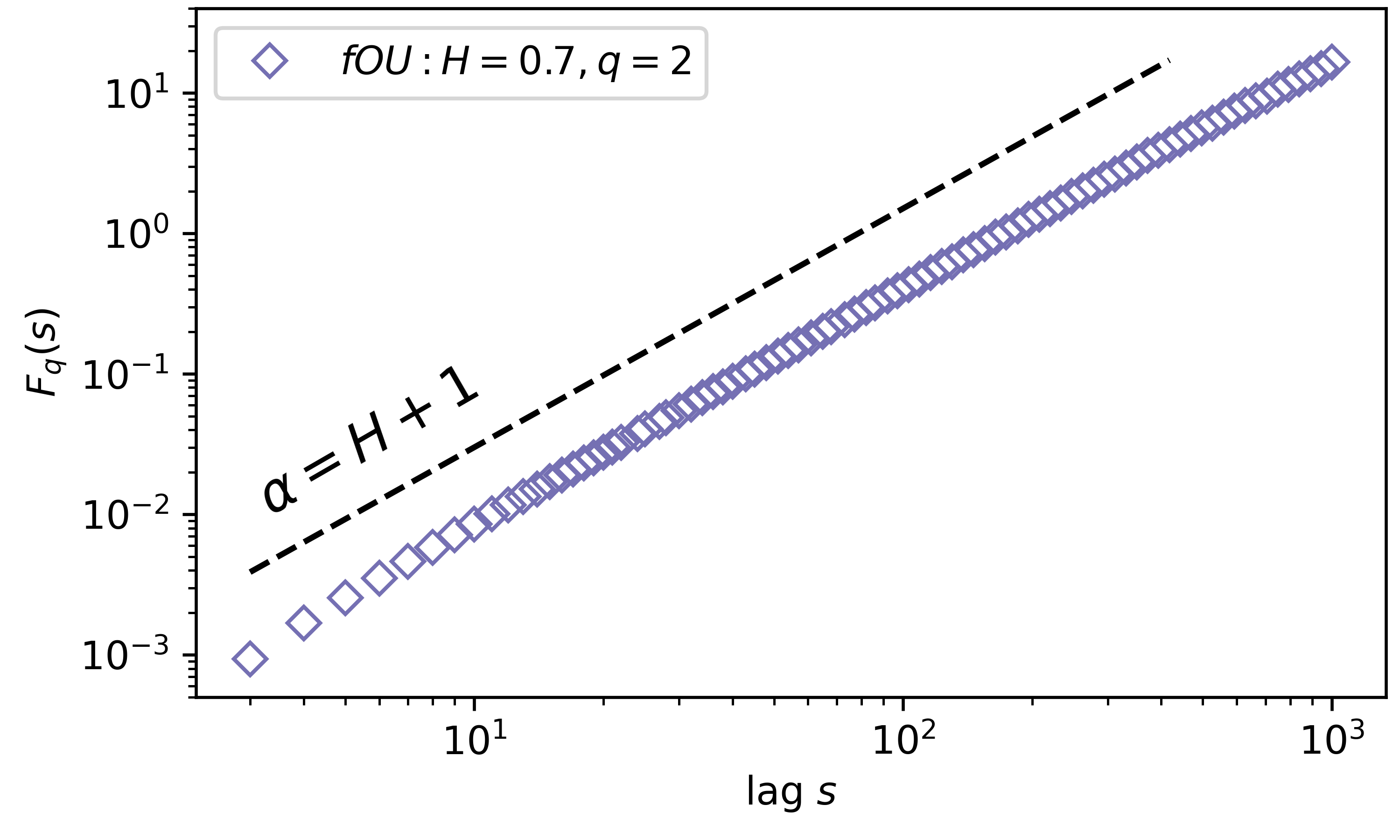
To now utilise the MFDFA, we take this exemplary process and run the (multifractal) detrended fluctuation analysis. For now lets consider only the monofractal case, so we need only $q = 2$.

# Select a band of lags, which usually ranges from
# very small segments of data, to very long ones, as
lag = np.unique(np.logspace(0.5, 3, 100, dtype=int))

# Notice these must be ints, since these will segment
# the data into chucks of lag size

# Select the power q
q = 2

# The order of the polynomial fitting
order = 1

# Obtain the (MF)DFA as
lag, dfa = MFDFA(y, lag = lag, q = q, order = order)

Now we need to visualise the results, which can be understood in a log-log scale. To find H we need to fit a line to the results in the log-log plot

# To uncover the Hurst index, lets get some log-log plots
plt.loglog(lag, dfa, 'o', label='fOU: MFDFA q=2')

# And now we need to fit the line to find the slope
# in a double logaritmic scales, i.e., you need to
# fit the logs of the results
H_hat = np.polyfit(np.log(lag)[4:20],np.log(dfa[4:20]),1)[0]

print('Estimated H = '+'{:.3f}'.format(H_hat[0]))


# Now what you should obtain is: slope = H + 1

$MFDFA of a fractional Ornstein–Uhlenbeck process$

Multifractality in one dimensional distributions¶

To show how multifractality can be studied, let us take a sample of random numbers of a symmetric Lévy distribution.

Univariate random numbers from a Lévy stable distribution¶

To obtain a sample of random numbers of Lévy stable distributions, use scipy’s levy_stable. In particular, take an $\alpha$-stable distribution, with $\alpha=1.5$

# Imports
from MFDFA import MFDFA
from scipy.stats import levy_stable

# Generate 100000 points
alpha = 1.5
X = levy_stable.rvs(alpha=alpha, beta = 0, size=10000)

For MFDFA to detect the multifractal spectrum of the data, we need to vary the parameter $q\in[-10,10]$ and exclude $0$. Let us also use a quadratic polynomial fitting by setting order=2

# Select a band of lags, which are ints
lag = np.unique(np.logspace(0.5, 3, 100).astype(int))

# Select a list of powers q
q_list = np.linspace(-10,10,41)
q_list = q_list[q_list!=0.0]

# The order of the polynomial fitting
order = 2

# Obtain the (MF)DFA as
lag, dfa = MFDFA(y, lag = lag, q = q_list, order = order)

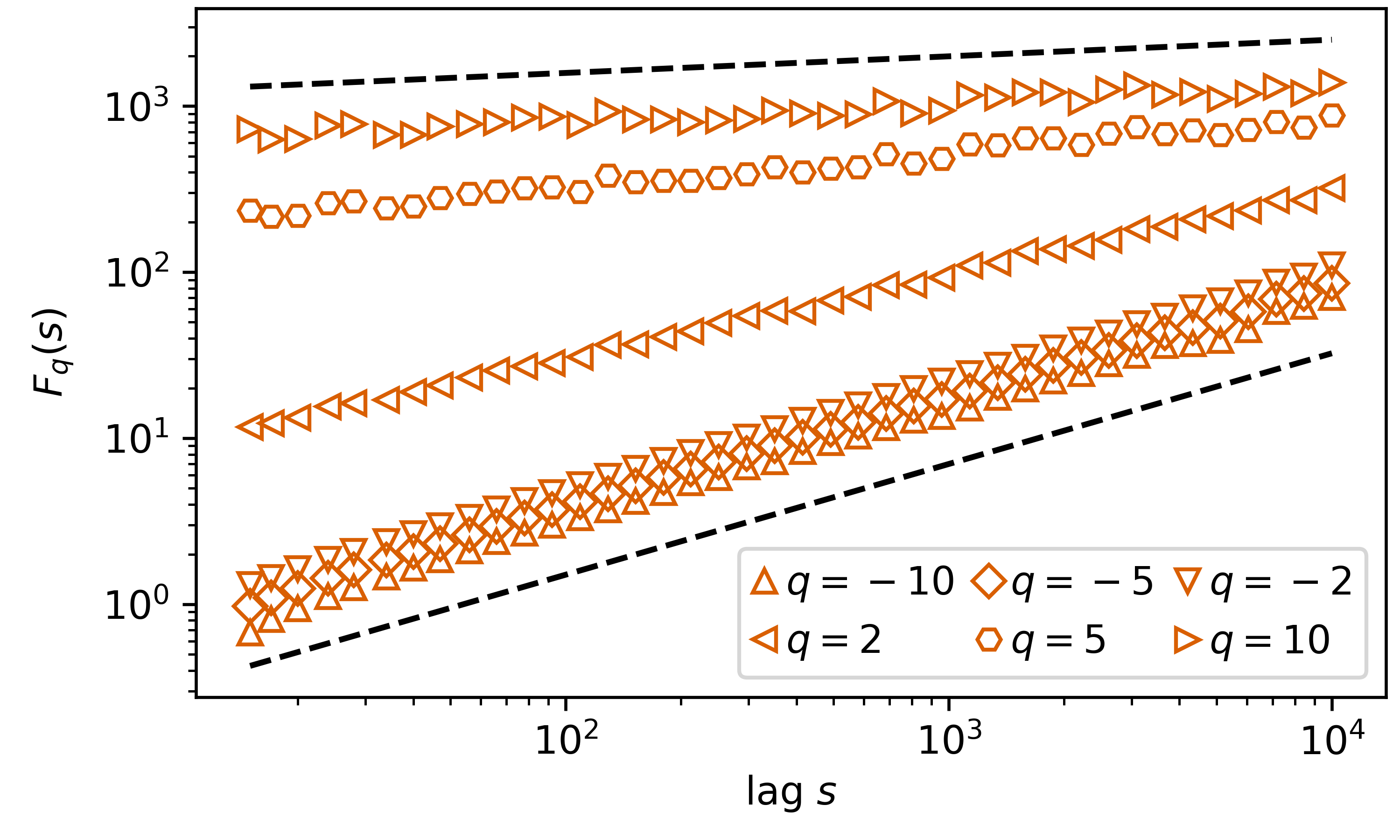
Again, we plot this in a double logarithmic scale, but now we include 6 curves, from 6 selected $q={-10,-5-2,2,5,10}$. Include as well are the theoretical curves for $q=-10$, with a slope of $1/\alpha=1/1.5$ and $q=10$, with a slope of $1/q=1/10$

Plot of the MFDFA of a Lévy stable distribution for a few q values.

Extensions¶

MFDFA as seen since its development a set of enhancements. In particular the usage of Empirical Mode Decomposition as a source of detrending, instead of polynomial fittings, which allows for a more precise removal of known trends in the timeseries.

Employing Empirical Mode Decompositions for detrending¶

Empirical Mode Decomposition (EMD), or maybe more correctly described, the Hilbert─Huang transform is a transformation analogous to a Fourier or Hilbert transform that decomposes a one-dimensional timeseries or signal into its Intrinsic Mode Functions (IMFs). For our purposes, we simply want to employ EMD to detrend a timeseries.

Warning

To use this feature, you need to first install PyEMD (EMD-signal) with

pip install EMD-signal

Understanding `MFDFA`’s `EMD` detrender¶

Take a timeseries y and extract the Intrinsic Mode Functions (IMFs)

# Import
from MFDFA import IMFs

# Extract the IMFs simply by employing
IMF = IMFs(y)

From here one obtains a (..., y.size). Best now to study the different IMFs is to plot them and the timeseries y

# Import
import matplotlib.pyplot as plt

# Plot the timeseries and the IMFs 6,7, and 8
plt.plot(X, color='black')
plt.plot(np.sum(IMF[[6,7,8],:], axis=0).T)

Using `MFDFA` with `EMD`¶

To now perform the multifractal detrended fluctuation analysis, simply insert the IMFs desired to be subtracted from the timeseries. This will also for order = 0, not to do any polynomial detrending.

# Select a band of lags, which usually ranges from
# very small segments of data, to very long ones, as
lag = np.logspace(0.7, 4, 30).astype(int)

# Obtain the (MF)DFA by declaring the IMFs to subtract
# in a list in the dictionary of the extensions
lag, dfa = MFDFA(y, lag = lag, extensions = {"EMD": [6,7,8]})

Extended Detrended Fluctuation Analysis¶

In the publication Detrended fluctuation analysis of cerebrovascular responses to abrupt changes in peripheral arterial pressure in rats. the authors introduce a new metric similar to the conventional Detrended Fluctuation Analysis (DFA) which they denote Extended Detrended Fluctuation Analysis (eDFA), which relies on extracting the difference of the minima and maxima for each segmentation of the data, granting a new power-law exponent to study, i.e., as in eq. (5) in the paper

\[\mathrm{d}F (n) = \mathrm{max}[F(n)] - \mathrm{min}[F(n)],\]

which in turn results in

\[\mathrm{d}F(n) \sim n^\beta.\]

Using `MFDFA`’s `eDFA` extension¶

To obtain the eDFA, simply set the extension to True and add a new output function, here denoted edfa

# Select a band of lags, which usually ranges from
# very small segments of data, to very long ones, as
lag = np.logspace(0.7, 4, 30).astype(int)

# Obtain the (MF)DFA by declaring the IMFs to subtract
# in a list in the dictionary of the extensions
lag, dfa, edfa = MFDFA(y, lag = lag, extensions = {'eDFA': True})

Moving window for segmentation¶

For short timeseries the segmentation of the data—especially for large lags—results in bad statistics, e.g. if a timeseries has 2048 datapoints and one wishes to study the flucutation analysis up to a lag of 512, only 4 segmentations of the data are possible for the lag 512. Instead one can use an moving window over the timeseries to obtain better statistics at large lags.

Using `MFDFA`’s `window` extension¶

To utilise a moving window one has to declare the moving windows step-size, i.e., the number of data points the window will move over the data. Say we wish to increase the statistics of the aforementioned example to include a moving window moving 32 steps (so one has 64 segments at a lag of 512)

# Select a band of lags, which usually ranges from
# very small segments of data, to very long ones, as
lag = np.logspace(0.7, 4, 30).astype(int)

# Obtain the (MF)DFA by declaring the IMFs to subtract
# in a list in the dictionary of the extensions
lag, dfa, edfa = MFDFA(y, lag = lag, extensions = {'window': 32})

Literature¶

¹ Peng, C.-K., Buldyrev, S. V., Havlin, S., Simons, M., Stanley, H. E., & Goldberger, A. L. (1994). Mosaic organization of DNA nucleotides. Physical Review E, 49(2), 1685–1689

² Kantelhardt, J. W., Zschiegner, S. A., Koscielny-Bunde, E., Havlin, S., Bunde, A., & Stanley, H. E. (2002). Multifractal detrended fluctuation analysis of nonstationary time series. Physica A: Statistical Mechanics and Its Applications, 316(1-4), 87–114

Funding¶

Helmholtz Association Initiative Energy System 2050 - A Contribution of the Research Field Energy and the grant No. VH-NG-1025, STORM - Stochastics for Time-Space Risk Models project of the Research Council of Norway (RCN) No. 274410, and the E-ON Stipendienfonds.