An exemplary one-dimensional fractional Ornstein–Uhlenbeck process

For a more detailed explanation on how to integrate an Ornstein–Uhlenbeck process, see the kramersmoyal’s package You can also follow the fOU.ipynb

Generating a fractional Ornstein–Uhlenbeck process

This is one method of generating a (fractional) Ornstein–Uhlenbeck process with \(H=0.7\), employing a simple Euler–Maruyama integration method

# Imports
from MFDFA import MFDFA
from MFDFA import fgn
# where this second library is to generate fractional Gaussian noises

# integration time and time sampling
t_final = 500
delta_t = 0.001

# Some drift theta and diffusion sigma parameters
theta = 0.3
sigma = 0.1

# The time array of the trajectory
time = np.arange(0, t_final, delta_t)

# The fractional Gaussian noise
H = 0.7
dB = (t_final ** H) * fgn(N = time.size, H = H)

# Initialise the array y
y = np.zeros([time.size])

# Integrate the process
for i in range(1, time.size):
   y[i] = y[i-1] - theta * y[i-1] * delta_t + sigma * dB[i]

And now you have a fractional process with a self-similarity exponent \(H=0.7\)

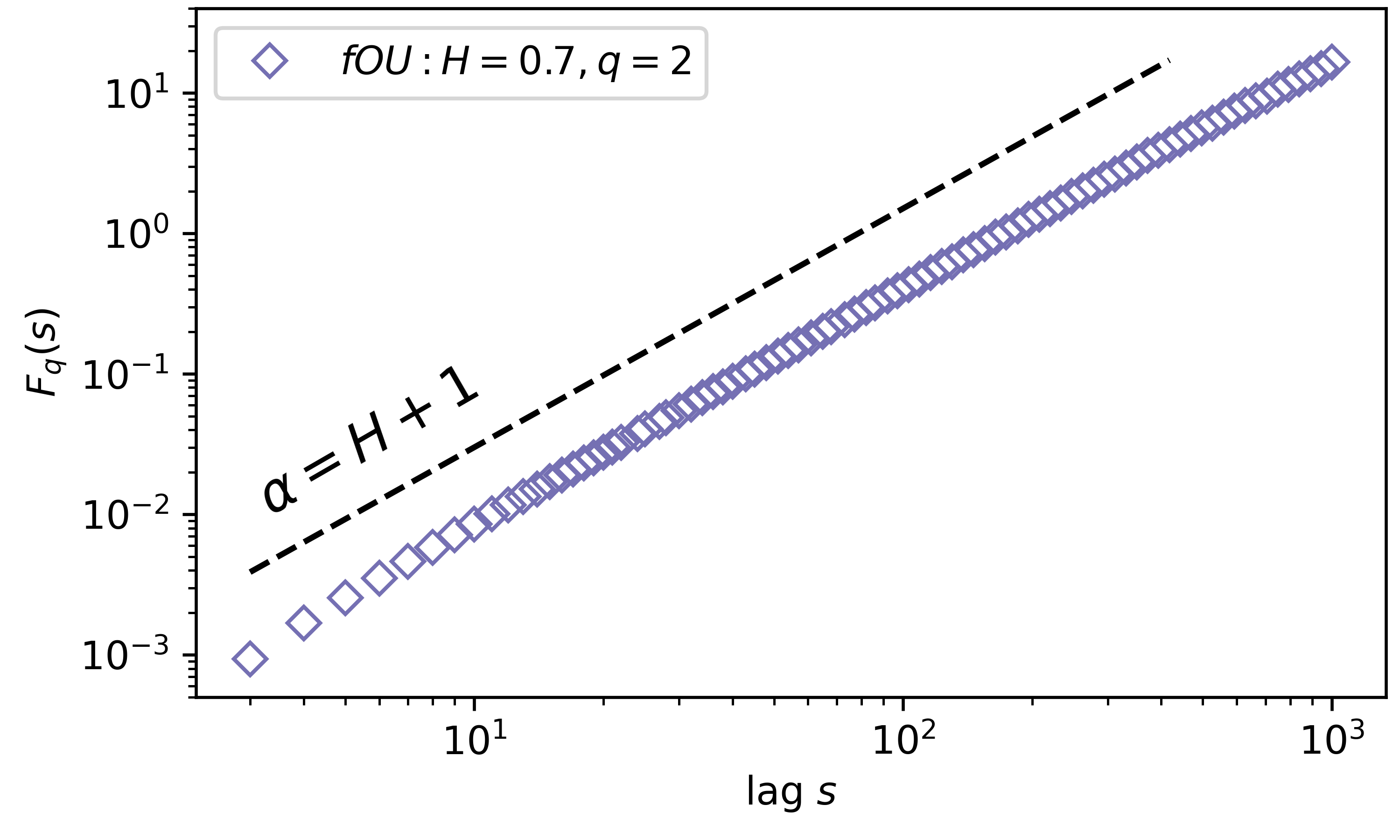
Using the MFDFA

To now utilise the MFDFA, we take this exemplary process and run the (multifractal) detrended fluctuation analysis. For now lets consider only the monofractal case, so we need only \(q = 2\).

# Select a band of lags, which usually ranges from
# very small segments of data, to very long ones, as
lag = np.unique(np.logspace(0.5, 3, 100, dtype=int))

# Notice these must be ints, since these will segment
# the data into chucks of lag size

# Select the power q
q = 2

# The order of the polynomial fitting
order = 1

# Obtain the (MF)DFA as
lag, dfa = MFDFA(y, lag = lag, q = q, order = order)

Now we need to visualise the results, which can be understood in a log-log scale. To find H we need to fit a line to the results in the log-log plot

# To uncover the Hurst index, lets get some log-log plots
plt.loglog(lag, dfa, 'o', label='fOU: MFDFA q=2')

# And now we need to fit the line to find the slope
# in a double logaritmic scales, i.e., you need to
# fit the logs of the results
H_hat = np.polyfit(np.log(lag)[4:20],np.log(dfa[4:20]),1)[0]

print('Estimated H = '+'{:.3f}'.format(H_hat[0]))


# Now what you should obtain is: slope = H + 1